Positional Embeddings
What are positional embeddings and why do we need them?
Transformers process token embeddings in parallel, so they have no context on the order of the tokens. The same token that appears in two different positions in a sequence will have the same embedding, which hinders the ability to understand text. For example, the text "The dog chased the cat" and "The cat chased the dog" would be interpreted the same since they have the same tokens. The solution to this is to add positional embeddings, information about tokens' positions so transformers can have context of the order of tokens in a sequence.
There are two main types of positional embeddings, absolute and relative. Absolute embeddings refer to a token's position in the sequence, and relative embeddings refer to the distance between two tokens relative to each other. I will cover both in this writing.
Lastly, before I cover different positional encoding methods, I will define the term extrapolation which will be used a lot. Extrapolation in this context refers to the model's ability to perform well on input sequences longer than seen in training.
Classic Sinusoidal Embeddings
Classic sinusoidal embeddings were used in the original transformer architecture, and add fixed sine and cosine functions of varying frequencies directly to the input token embeddings.
For a given sequence position pos and a dimension index i (where i ranges from 0 to dmodel/2 − 1), the positional embeddings are calculated using the following formulas:
Even dimensions:  PE(pos, 2i)   = sin( pos / 10000^(2i / d_model) )
Odd  dimensions:  PE(pos, 2i+1) = cos( pos / 10000^(2i / d_model) )
Key Variables:
- pos: The position of the token in the sequence (e.g., 0, 1, 2…).
- i: The index of the dimension within the embedding vector.
- dmodel: The total dimensionality of the model's embeddings (e.g., 512).
Strengths
- Fixed, no parameters to learn.
- Predictable nature of sine and cosine functions allow the model to generalize, resulting in good extrapolation, although ALiBi came out with findings that it does not extrapolate as well as previously believed.
Weaknesses
- Can't adapt to specific data well.
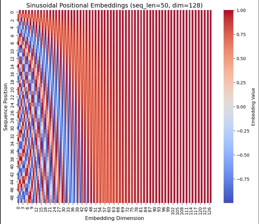
Sinusoidal positional encoding heatmap. High-frequency waves on the left, low-frequency waves on the right.
In this visualization you can observe the colors rapidly changing on the left side representing high-frequency waves, and not changing much as you look to the right representing low-frequency waves. The key idea when thinking about position is that each row represents a positional embedding vector, and each embedding has a unique "id". We can't use single integers to model positions at a large scale, but this method handles large amounts of data because using sine and cosine keeps all values between −1 and 1.
To calculate the similarity of two tokens' positions from these embeddings we can take the dot product of the two, visualized in the following plot.
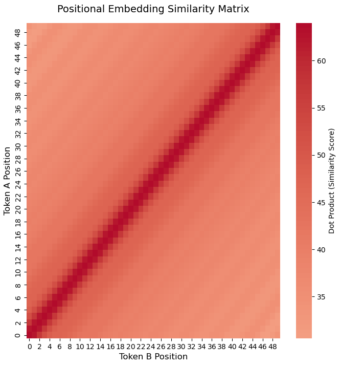
Sinusoidal positional similarity matrix showing gradual similarity decrease as token distance increases.
The similarity matrix visualized shows the gradual fading of color away from the diagonal, and a decrease in similarity value as the two tokens' positions get further apart.
Learned Embeddings
Learned embeddings were used in the GPT-2 and GPT-3 models, and treat position embeddings similarly to tokens. They randomly initialize a vector of the same size as the token embedding vector. Unlike sinusoidal embeddings which are frozen (not updated during training), these learned positional embeddings are updated during training to give context of the position of each token.
Strengths
- Adaptable to specific datasets.
Weaknesses
- Fixed max sequence length, does not extrapolate well.
- More parameters to be learned, resulting in longer and more intensive training.
Rotary Positional Embeddings (RoPE)
Instead of adding the positional embedding to the token embedding vector, RoPE introduces a rotation operation to encode the positional information directly into the attention mechanism. It takes the query and key vectors and physically rotates them in a multi-dimensional space, with the angle of rotation determined by the token's absolute position index. This operation is done before the multiplication happens in the attention mechanism.
The math behind RoPE is complex, but essentially it works because trig identities cause the absolute angles to cancel out after the dot product of the two rotated vectors is computed. The resulting attention score is determined only by the difference in their angles, corresponding to the relative distance between tokens.
RoPE captures the relative distance between tokens, compared to the two previous absolute embedding methods. Due to rotation's periodic nature, RoPE performs well on extrapolation to input sequences longer than seen during training. Because of this, RoPE is used in many frontier models like Llama, Mistral, Gemini, and Claude. It is known to not perform well on sequences much larger than seen during training, but there have been new tricks discovered as a solution to this problem, such as YaRN and linear interpolation.
Strengths
- Integrates positional information directly into attention.
- Extrapolates well due to rotation's periodic nature.
Weaknesses
- Complex math to implement.
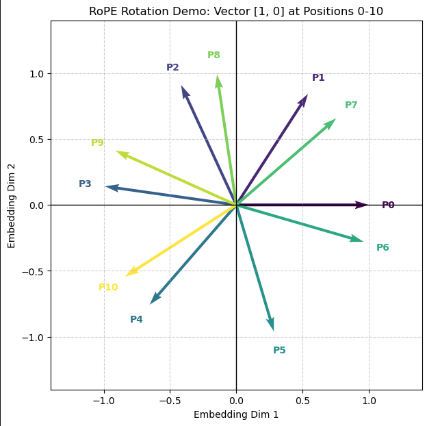
RoPE applied to the same 2D token embedding across 11 positions. Each vector has the same magnitude, and adjacent vectors have the same angle between them.
The above example illustrates RoPE applied on the same 2D token embedding in 11 different positions, so that the only differentiation between them is their position. We can see that each vector has the same magnitude since they all represent the same token, and each adjacent vector has the same angle between them, showing how it is only based on the distance between tokens.
Attention with Linear Biases (ALiBi)
ALiBi introduces a new concept, not using positional embeddings at all. ALiBi adds a static penalty bias directly to query-key attention scores after multiplication. This penalty is proportional to the distance between query and key, and favors tokens that are closer together.
Strengths
- Extrapolates very well.
- Eliminates the use of embeddings.
- Simple implementation.
Weaknesses
- Distant tokens are largely ignored due to the penalty bias.
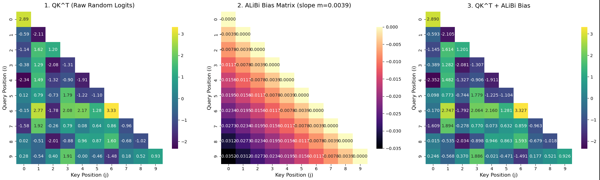
Three-panel ALiBi visualization: semantic similarity (left), bias matrix (center), ALiBi-adjusted scores (right).
Plot 1: Does not have any positional context, shows only semantic similarity between tokens.
Plot 2: Shows the bias matrix. When i = j the penalty is 0, but as the token distance increases, the penalty increases (darker colors). You can see this at query position 9 and key position 0, the darkest value because the tokens are furthest apart.
Plot 3: ALiBi bias applied. Tokens along and near the diagonal are unchanged or minimally affected because there is no or small penalty. Values at positions further apart are changed more because they receive a higher penalty.
3D Demo
3D animation of sinusoidal positional embeddings built with the manim library.
I created this 3D animation of sinusoidal embeddings being applied using the manim library. You can see that with only token embeddings, the two instances of 'cat' have the same vector, but adding positional embeddings is what differentiates them.
Ablation Study
Here is a study where I dropped positional embeddings from an attention mechanism and visualized how it affected the attention weights afterwards.
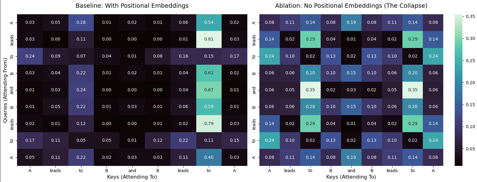
Left: attention weights with positional embeddings. Right: attention weights without positional embeddings.
The plots show exactly why positional embeddings are so important. In the left plot, you can see that the same words in different positions have different attention weights, so they are treated differently depending on their position in the sequence. The plot on the right shows the values with positional embeddings ablated, instances of the same token in different positions have the exact same attention weights.
Conclusion
For each of these methods, I researched, implemented, and created demos for them. You can see more about the implementation in the Jupyter notebook in the linked GitHub repository. The method that interested me the most was ALiBi, and I am interested to see if new advancements will be made to it so more models pick it up.
References
- https://towardsdatascience.com/positional-embeddings-in-transformers-a-math-guide-to-rope-alibi/
- https://medium.com/autonomous-agents/math-behind-positional-embeddings-in-transformer-models-921db18b0c28
- https://machinelearningmastery.com/positional-encodings-in-transformer-models/
- https://arxiv.org/pdf/1706.03762
- https://arxiv.org/pdf/2104.09864
- https://arxiv.org/pdf/2108.12409